Engineering a Nowcasting System using Open Data Sources
Introduction
Water vapor plays an important role in the atmosphere as it holds water in the vapor form which is capable of traveling both horizontally and vertically over a short span of time. This movement of water vapor greatly affect the weather in a vary short time scale (the next few hours). Thus by measuring this quantity with sufficient spatial and temporal resolution we can understand and predict severe storms better.
Water vapor is also a difficult quantity to measure and some of the existing methods do not capture its temporal and spatial variability required for operational forecasting. Some of the existing techniques to measure water vapor is as follows.
-
Radiosondes: A radiosonde is a battery powered telemetry instrument package with sensors for sampling various atmospheric variables as it is carried up by a balloon from ground launch to between 20-30 km altitude (http://www.wrh.noaa.gov/rev/tour/UA/introduction.php). While radiosondes have the advantage that they can measure the vertical distribution of water vapor, they have the distinct disadvantages that they are typically only launched two times a day (at 0000 and 1200 UTC) and from only a handful of locations (the entire CONUS is covered by a mere 90 radiosonde launch sites).
-
Radiometers: Ground-based water vapor radiometers measure the background microwave radiation emitted by atmospheric water vapor along a given line of site. An advantage of these instruments is their ability to make continuous measurements of water vapor. Disadvantages are cost, calibration, and sparse spatial deployment. They are also limited in that they do not work when it is raining.
-
Satellites: The GOES (Geostationary Operational Environmental Satellite) system provides two sources of information about the water vapor imagery through its water vapor channel (at 4km spatial resolution, 15 min temporal resolution), and sounder retrievals (at 20km spatial resolution, 1hr temporal resolution). Both of these observations, however, are negatively impacted by cloud cover.
-
GPS-Meteorology: GPS-meteorology (GPS-Met) is a technique that allows GPS receivers to simultaneously perform the multiple functions of position estimation and precipitable water vapor estimation. For a given GPS receiver, precipitable water vapor estimates can be made with 30-minute temporal resolution. In regions, such as the middle and western U.S., where there is a high density of Continuously Operated GPS Reference Stations (CORS). Techniques have been developed to combine the water vapor measurements from multiple stations into 2D and 3D water vapor fields. The spatial resolution of the field depends on the density of GPS stations (spatial Nyquist). While GPS-Met currently cannot provide the spatial and temporal resolution of that of GOES satellite, it has the advantage that it is accurate in all weather conditions and not impacted by clouds or precipitation.
Our solution for the Vaisala Open Weather data challenge is focused on using open source GNSS data from a dense network of GNSS stations along with in-situ surface meterological observations to obtain a the amount of precipitable water vapor in the atmosphere. Using the water vapor derived from a network of GNSS stations and precipitation products from weather radars, our goal is to develop a nowcasting system which integrates this data from open data sources and nowcasts precipitation.
Data and Software
This section explains all of our data sources and open source software packages used in our data pipeline.
Open Source Data
-
GNSS(Global Navigation Satellite Systems) data: High precision GNSS signals from dual frequency receivers which operate continuously are in the form of RINEX (Receiver Independent Exchange format) files. These files contain pseudo range and carrier phase data from each satellite in view at 30s intervals. For over a 1000 stations world wide RINEX files can be obtained from FTP servers maintained by organizations such as NOAA NGS CORS(Continuously Operated Reference Stations), SOPAC (Scripps Orbit and Permanent Array Center), IGS (International GNSS Services).
Real time data: The above mentioned servers also provide realtime data of the RINEX files for select stations. -
Meteorological data: Since most of the GNSS stations in our study do not have co-located weather stations we interpolate the meterological observations from a network of weather stations operated by NOAA NWS called ASOS(Automates Surface Observing Systems). These stations record pressure, relative humidity and temperature in 30 minute intervals. After extensively searching the web for the meteorological data from ASOS stations in the 30 minute intervals, we obtained the data for the entire year of 2014 from Dr. Teresa Van Hove from UCAR COSMIC (Constellation Observing System for Meteorology, Ionosphere, and Climate) program. We downloaded the meteorological data for the year 2014 for select stations from a UCAR server from a link provided by Dr. Teresa Van Hove.
Real time data: The realtime feed from the ASOS stations is distributed thru the LDM protocol. Dr. Teresa also provided us with a LDM link so that we can get a feed of the real time ASOS data (suomildm1.cosmic.ucar.edu). -
NOAA NEXRAD reflectivity products: We obtain the level III radar reflectivity products from the NOAA NCDC archive.
Real time data: For real time operation we are developing a script which pulls the level II reflectivity products from NOAA NEXRAD reflectivity database on Amazon S3.
Open Source Software
We use freely available software to process and analyse our data.
-
GAMIT (GPS Analysis at MIT): The GAMIT software package takes in the input RINEX observation(carrier phase and pseudo range data) and meterological files and processes the IPW for each station.
-
Python: The development of our nowcasting system is in python and we use the machine learning library scikit-learn.
Data Pipeline
The data set we will use for our nowcasting experiments comes from the Dallas-Fort-Worth (DFW) region. Part of the infamous U.S. “tornado alley”, DFW spring and summer weather is dominated by convective thunderstorms that move in lines generally from west to east through the region. We choose the DFW region because we understand its climatology (through CASA’s more than 15 years of operating networks of weather radars in tornado alley, first in Oklahoma and now in DFW) and because the DFW region has a high density of GPS receivers and weather stations whose data are publicly available on-line for our use.
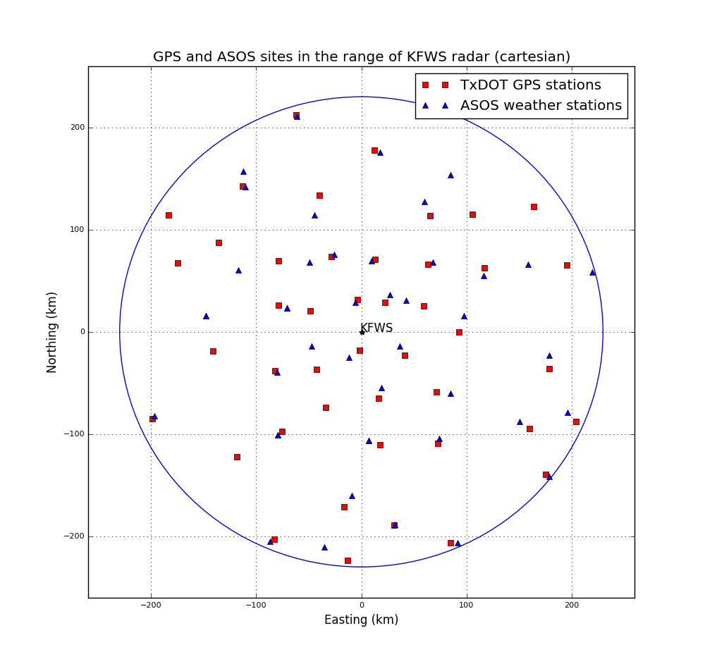
We take as the center of our domain the NWS KFWS NEXRAD radar in Fort-Worth Texas. Within the 230 km coverage range of the radar we identified 44 Regional Reference Points, i.e., high performance dual-frequency GPS receivers. We found these stations by parsing through GNSS station log files and identified the stations which are within the 230 km range radius ot the radar. Further we found out that most of these GNSS receivers are operated by the Texas Dept. of Transportation (TxDOT), and were deployed to provide precise position information for Geodetic studies. As such these GNSS receivers do not have collocated weather stations. For the weather data (surface temperature, pressure, and relative humidity) required for IPW estimation, we used data from the network of Automated Surface Observation Stations (ASOS) operated by NOAA NWS. We find the closest ASOS station to each GNSS station and interpolate the meteorological variables from the MSL of the ASOS station to the MSL of the GNSS station as suggested by (Bai et al 2003). The near real-time water vapor system operated by UCAR follows a similar principle. The figure below shows a map of all the sensors used in this study with respect to the KFWS radar in Dallas Fort Worth.
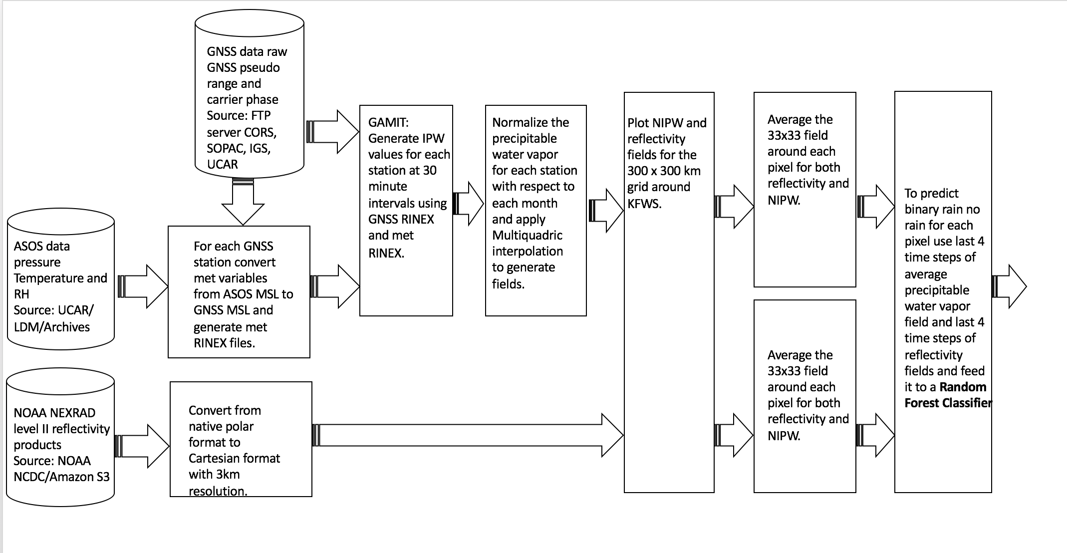
The following figure summarizes the data pipeline which includes all of out input data bases to our output products.
Preliminary Experiments
From the data sources listed above we obtain the GNSS RINEX files for all 44 stations, met observations from 40 ASOS stations for the entire year of 2014. We then feed the RINEX observation files (containing pseudo range and carrier phase) and RINEX met data (containing pressure, temperature and relative humidity for each station) to the GAMIT software to obtain 30 minute intervals of precipitable water vapor measurements for each station for the entire year of 2014.
We then normalize the precipitable water vapor with respect to each station and month. This mainly serves two purposes one the measured water vapor will be different measured by GNSS stations at different heights and second the atmosphere can hold different amounts of water vapor at different times of the year. We then select 23 days from the storm season (May-August) in 2014 for our training/test set for our machine learning experiments. We choose days which have normalized precipitable water vapor values exceeding 2 standard deviations from normal and term these days as “Weather Anomalies”.
We use the Multiquadric Interpolation technique suggested by (Tabios et al. 1985) to interpolate the point measurements of normalized precipitable water vapor to a field spaning 300 by 300 km centered on the KFWS radar with a resolution of 3km. The reflectivity fields are also converted from its native polar coordinates to cartesian coordinates to match the resolution of the precipitable water fields. The following video shows the reflectivity fields overlapped over the normalized precipitable water fields for a storm case on May 8th 2014 UTC.
Our initial machine learning experiment is to learn Random Forest Classifier to predict rain or no rain(rain defined as pixel points exceeding 24 dbZ) 1 hour into the future for each pixel based on the last 4 time steps of precipitable water vapor and reflectivity fields at 30 minute intervals. As an initial step we crop the 33 by 33 field around each pixel for both the fields and average them which are features for our random forest classifier.
The random forest is trained and tested using a K-fold cross validation technique from the above mentioned 23 days. We perform 3 sets of experiments as follows:
- Use precipitable water features only
- Use reflectivity features only
- Use both precipitable water and reflectivity features.
The results of the above three experiments are evaluated using a precision recall curve as shown below.
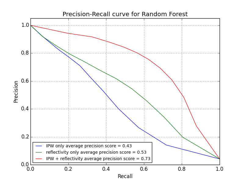
As seen by the precision recall curves we can observe that the average precision score (area under the curve) evaluated by varying the decision probability for the IPW and reflectivity feature is the highest. The random forest classifier thus performs best when IPW features are concatenated with the reflectivity features. The following table shows additional metrics for our nowcasting algorithm where POD is Probability of Detection, FAR is False Alarm Rate and CSI is Critical Success Index.
| IPW | Refl. | IPW + Refl. | |
|---|---|---|---|
| POD | 0.17 | 0.38 | 0.56 |
| FAR | 0.23 | 0.29 | 0.15 |
| CSI | 0.16 | 0.33 | 0.51 |
Conclusion and Discussion
In this solution we propose to build a data pipeline which integrates data from 3 different sources for a given region. We further used a random forest classifier to predict the precipitation fields 1 hour into the future. There is room for a lot of improvement in our system. Our data pipeline is modular and thus a single block can be optimized independently to improve the performance of the system. We measure performance of the nowcasting system using precision recall curves and standard nowcasting metrics such as POD, FAR and CSI.
Our next step is to to build a feature engineering module which extracts the features from the precipitable water vapor fields and the precipitation fields to predict the precipitation fields 1 hour in the future. We also plan to deploy our system in real time before the storm season of 2016.